| (1) |
| (1) |
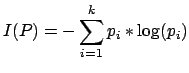
In general, if we are given a probability
distribution
![]() then the Information conveyed by this
distribution (also called the Entropy of P), is:
then the Information conveyed by this
distribution (also called the Entropy of P), is:
For example, if ![]() is
is
![]() then
then ![]() is 1, if P is
is 1, if P is
![]() then
then ![]() is 0.92, if P is
is 0.92, if P is ![]() then
then ![]() is 0. [Note that the more uniform is the probability distribution,
the greater is its information.]
is 0. [Note that the more uniform is the probability distribution,
the greater is its information.]
An other example: We want to known if a golfer will play or not based on the following data:
    OUTLOOK | TEMPERATURE | HUMIDITY | WINDY | PLAY
    =====================================================
    sunny   |      85     |    85    | false | Don't Play
    sunny   |      80     |    90    | true  | Don't Play
    overcast|      83     |    78    | false | Play
    rain    |      70     |    96    | false | Play
    rain    |      68     |    80    | false | Play
    rain    |      65     |    70    | true  | Don't Play
    overcast|      64     |    65    | true  | Play
    sunny   |      72     |    95    | false | Don't Play
    sunny   |      69     |    70    | false | Play
    rain    |      75     |    80    | false | Play
    sunny   |      75     |    70    | true  | Play
    overcast|      72     |    90    | true  | Play
    overcast|      81     |    75    | false | Play
    rain    |      71     |    80    | true  | Don't Play
We will build a classifier which, based on the features OUTLOOK, TEMPERATURE,
HUMIDITY and WINDY will predict wether or not the golfer will play. There
are 2 classes: (play) and (don't play). There are 14 examples. There are 5
examples which gives as result "don't play" and 9 examples which gives as
result "will play."
We will thus have
![]()
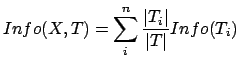
Consider a similar measurement after ![]() has been partitioned in
accordance with the
has been partitioned in
accordance with the ![]() outcomes of a test on the feature X. (in
the golfer example, X can be a test on OUTLOOK, TEMPERATURE, ...).
The expected information requirement can be found as a weighted
sum over the subsets:
outcomes of a test on the feature X. (in
the golfer example, X can be a test on OUTLOOK, TEMPERATURE, ...).
The expected information requirement can be found as a weighted
sum over the subsets:
In the case of our golfing example, for the attribute Outlook we have:
| (5) |
Consider the quantity ![]() defined as:
defined as:
| (6) |
This represents the difference between the information needed to
identify an element of T and the information needed to identify an
element of T after the value of attribute X has been obtained,
that is, this is the gain in information due to attribute X.
In our golfing example, for the Outlook attribute the gain is:
| (7) |
If we instead consider the attribute Windy, we find that
![]() . Thus
OUTLOOK offers a greater informational gain than WINDY.
. Thus
OUTLOOK offers a greater informational gain than WINDY.
We can use this notion of gain to rank attributes and to build
decision trees where at each node is located the attribute with
greatest gain among the attributes not yet considered in the path
from the root.
In the Golfing example we will obtain the following decision tree:
                        Outlook
                       / |     \
                      /  |      \
            overcast /   |sunny  \rain
                    /    |        \
               Play    Humidity   Windy
                     /   |         |  \
                    /    |         |   \
              <=75 /  >75|     true|    \false
                  /      |         |     \
                 Play   Don'tPlay Don'tPlay Play
The notion of Gain introduced earlier tends to favor test on
features that have a large number of outcomes (when ![]() is big in
equation 4). For example, if we have a feature
is big in
equation 4). For example, if we have a feature ![]() that
has a distinct value for each record, then
that
has a distinct value for each record, then ![]() is 0, thus
is 0, thus
![]() is maximal. To compensate for this Quinlan suggests
using the following ratio instead of Gain:
is maximal. To compensate for this Quinlan suggests
using the following ratio instead of Gain:
GainRatio(X,T)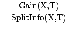 |
(8) |
Consider the information content of a message that indicate not
the class to which the case belongs, but the outcome of the test
on feature ![]() . By analogy with equation 3, we have
. By analogy with equation 3, we have
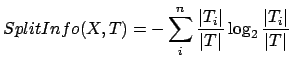 |
(9) |
The
![]() is thus the proportion of information generated by the
split that is useful for the classification.
is thus the proportion of information generated by the
split that is useful for the classification.
In the case of our golfing example
![]() and
and
![]() .
.
We can use this notion of ![]() to rank attributes and to
build decision trees where at each node is located the attribute
with greatest
to rank attributes and to
build decision trees where at each node is located the attribute
with greatest ![]() among the attributes not yet considered
in the path from the root.
among the attributes not yet considered
in the path from the root.
We can also deal with the case of features with continuous ranges.
Say that feature ![]() has a continuous range. We examine the values
for this features in the training set. Say they are, in increasing
order,
has a continuous range. We examine the values
for this features in the training set. Say they are, in increasing
order,
![]() . Then for each value
. Then for each value
![]() we partition the records into 2 sets : the first set
have the
we partition the records into 2 sets : the first set
have the ![]() values up to and including
values up to and including ![]() and the second set
have the
and the second set
have the ![]() values greater than
values greater than ![]() . For each of these
. For each of these ![]() partitions we compute the
partitions we compute the
![]() , and
choose the partition that maximizes the gain. If all features are
continuous, we will obtain a binary tree.
, and
choose the partition that maximizes the gain. If all features are
continuous, we will obtain a binary tree.
Pruning a tree is the action to replace a whole subtree by a leaf.
The replacement takes place if the expected error rate in the
subtree is greater than in the single leaf. We will start by
generating the whole (generally overfitted) classification tree
and simplify it using pruning just after.
The error estimates for leaves and subtrees are computed assuming
that they were used to classify a set of unseen cases of the same
size as the training set. So a leaf covering ![]() training cases
(
training cases
(![]() of them incorrectly) with a predicted error rate of
of them incorrectly) with a predicted error rate of
![]() (with
(with ![]() : the binomial distribution,
: the binomial distribution, ![]() : the
Confidence Level) would give rise to a predicted
: the
Confidence Level) would give rise to a predicted
![]() errors. Similarly, the number of predicted errors
associated with a (sub)tree is just
the sum the the predicted errors of its branches.
errors. Similarly, the number of predicted errors
associated with a (sub)tree is just
the sum the the predicted errors of its branches.
An example: Let's consider a dataset of 16 examples describing
toys. We want to know if the toy is fun or not.
    COLOR   | MAX NUMBER OF PLAYERS | FUN
    =====================================================
    red     |  2                    | yes
    red     |  3                    | yes
    green   |  2                    | yes
    red     |  2                    | yes
    green   |  2                    | yes
    green   |  4                    | yes
    green   |  2                    | yes
    green   |  1                    | yes
    red     |  2                    | yes
    green   |  2                    | yes
    red     |  1                    | yes
    blue    |  2                    | no
    green   |  2                    | yes
    green   |  1                    | yes
    red     |  3                    | yes
    green   |  1                    | yes
We obtain the following classification tree:
                   Color
                /    |     \
               /     |      \             pruning
          red /      |green  \blue   =================>    yes
             /       |        \
            yes     yes       no
          (leaf1)  (leaf2)   (leaf3)
The predicted error rate for leaf 1 is
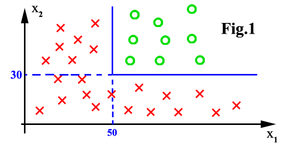
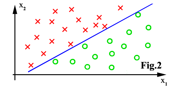
The major limitation is that the feature space can only be partitioned
in boxes parallel to axes of the space. There is no problem in figure 1,
above. There will be bad classification accuracy in figure 2.
We can use many classifiers and make a vote to obtain the final
class of the examples we want to classify. How does it help? Let's
assume you have 10 decision trees
How to generate the 10 trees? We don't have to know what are the
specialty of each tree. We only have to build trees that have
various behavior. We will build the 10 different trees using the
algorithm previously described on 10 different sets of examples.
How do we generate these 10 sets of example? We will use only a
small part (called a bootstrap) of the full set of example (this
technique is called BAGGING). Each bootstrap (there are here 10)
will be build using random example taken from the full set of
example (random selection with duplication allowed). We will also
use a small subset of all the features available (this technique
is called FEATURE SELECTION). For each bootstrap, we will use
different randomly chosen features (random selection with
duplication forbidden). The combination of BAGGING
and FEATURE SELECTION is called BAGFS.
What's the optimal number of trees? Can we take the highest number
possible? no, because another phenomena will appear: the
OVERFITING. The classifier lose its generalization ability. It can
only classify the examples which were used to build it. It cannot
classify correctly unseen examples.
![]() . The predicted error rate for leaf 2 is
. The predicted error rate for leaf 2 is
![]() . The predicted error rate for leaf 3
is
. The predicted error rate for leaf 3
is
![]() . The total number of
predicted error for this subtree is
. The total number of
predicted error for this subtree is
![]() . If the tree were replaced by the
simple leaf "Yes", the predicted error rate would have been:
. If the tree were replaced by the
simple leaf "Yes", the predicted error rate would have been:
![]() . Since the simple
leaf has a lower predicted error (
. Since the simple
leaf has a lower predicted error (
![]() ), the tree is
pruned to a leaf.
), the tree is
pruned to a leaf.
Limitations
The implementation of the classification-tree algorithm I realized is only
able to classify continuous features. This means, that it
can only generate binary trees. We can still use the program with special
discrete features like MAX NUMBER OF PLAYERS=(1,2,3,4) in the toy
example above. We can use discrete features if they exhibit some ordering
property. This means that discrete features like COLOR=(red,green,blue)
are not allowed.
Bagging and Feature selection
![]() . You
want to make classification in 3 classes
. You
want to make classification in 3 classes
![]() . Let's
now assume that the first 4 trees
. Let's
now assume that the first 4 trees
![]() always
recognize and classify correctly class
always
recognize and classify correctly class ![]() (they are specialized
for
(they are specialized
for ![]() ). The other trees are specialized in other classes.
Let's now assume you want to classify a new example. This example
belongs to
). The other trees are specialized in other classes.
Let's now assume you want to classify a new example. This example
belongs to ![]() . The trees
. The trees
![]() will answer
will answer ![]() .
The other trees will gives random answer which will form some
"uniformly distributed noise" during the vote. The result of the
vote will thus be
.
The other trees will gives random answer which will form some
"uniformly distributed noise" during the vote. The result of the
vote will thus be ![]() . We just realized an error
de-correlation.
. We just realized an error
de-correlation.
Bibliography
The excellent book
of Quinlan.
 bits.
bits.