| (1) |
Let the world state at time
| (1) |
The objective is to find a policy ![]() , or rule for selecting
actions, so that the expected value of the return is maximized. It
is sufficient to restrict attention to policies that select
actions based only on the current state (called stationary
policies) :
, or rule for selecting
actions, so that the expected value of the return is maximized. It
is sufficient to restrict attention to policies that select
actions based only on the current state (called stationary
policies) :
![]() . For any such policy
. For any such policy ![]() and for any
state
and for any
state ![]() we define:
we define:
| (2) |
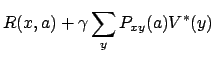
The expected total discounted return received when starting in
state x and following policy ![]() thereafter. If
thereafter. If ![]() is an
optimal policy we also use the notation
is an
optimal policy we also use the notation ![]() for
for ![]() . Many
dynamic programming-based reinforcement learning methods involve
trying to estimate the state values
. Many
dynamic programming-based reinforcement learning methods involve
trying to estimate the state values ![]() or
or ![]() for a
fixed policy
for a
fixed policy ![]() .
.
Q-learning, is a simple incremental algorithm developed from the
theory of dynamic programming [Ross,1983] for delayed
reinforcement learning. In Q-learning, policies and the value
function are represented by a two-dimensional lookup table indexed
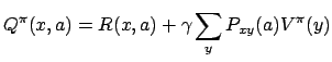
by state-action pairs. Formally, for each state ![]() and action
and action ![]() let:
let:
where
![]() and
and ![]() is
the probability of reaching state
is
the probability of reaching state ![]() as a result of taking action
as a result of taking action
![]() in state
in state ![]() . It follows that
. It follows that
| (5) |
 |
(6) |
The Q-learning algorithm works by maintaining an estimate of the
![]() function, which we denote by
function, which we denote by ![]() , and adjusting
, and adjusting
![]() values (often just called Q-values) based on
actions taken and reward received. This is done using Sutton's
prediction difference, or TD error [Sutton,1988] - the difference
between (the immediate reward received plus the discounted value
of the next state) and (the Q-value of the current state-action
pair):
values (often just called Q-values) based on
actions taken and reward received. This is done using Sutton's
prediction difference, or TD error [Sutton,1988] - the difference
between (the immediate reward received plus the discounted value
of the next state) and (the Q-value of the current state-action
pair):
| (7) |
where
![]() is a learning rate parameter. Note
that the current estimate of the
is a learning rate parameter. Note
that the current estimate of the ![]() function implicitly defines
a greedy policy by
function implicitly defines
a greedy policy by
![]() . That is, the greedy policy is to select actions
with the largest estimated
Q-value.
. That is, the greedy policy is to select actions
with the largest estimated
Q-value.
It is important to note that the Q-learning method does not
specify what actions the agent should take at each state as it
updates its estimates. In fact, the agent may take whatever
actions it pleases. This means that Q-learning allows arbitrary
experimentation while at the same time preserving the current best
estimate of states' values. This is possible because Q-learning
constructs a value function on the state-action space, instead of
the state space. It constructs a value function on the state space
only indirectly. Furthermore, since this function is updated
according to the ostensibly optimal choice of action at the
following state, it does not matter what action is actually
followed at that state. For this reason, the estimated returns in
Q-learning are not contaminated by "experimental" actions
[Watkins,1989], so Q-learning is not experimentation-sensitive.
To find the optimal Q function eventually, however, the agent must
try out each action in every state many times. It has been shown
[Watkins,1989 ; Dayan,1992] that if equation 8 is
repeatedly applied to all state-action pairs in any order in which
each state-action pair's Q-value is updated infinitely often, then
![]() will converge to
will converge to ![]() and
and ![]() will converge
to
will converge
to ![]() with probability 1 as long as
with probability 1 as long as ![]() is reduced to 0 at
a suitable rate. This is why the policy
is reduced to 0 at
a suitable rate. This is why the policy
![]() is only used a part of the time in order to be
able to explore the state-action space completely. At each
iteration
is only used a part of the time in order to be
able to explore the state-action space completely. At each
iteration ![]() , we will choose to make either a random action
, we will choose to make either a random action
![]() random or the optimal action
random or the optimal action
![]() . We
will take the first possibility (the random action) with a
probability of
. We
will take the first possibility (the random action) with a
probability of ![]() . At the beginning of the learning
. At the beginning of the learning
![]() must be huge (near 1). At the end of the learning, when
must be huge (near 1). At the end of the learning, when
![]() , we will set
, we will set
![]() to always use
the optimal policy. It is, as always, the compromise between
exploitation-exploration.
to always use
the optimal policy. It is, as always, the compromise between
exploitation-exploration.
Shortly, we have:
An illustration of these concepts is the robot example. At each time step,
the robot can choose one of the following action:
The reward ![]() the robot gets is simply the number of pixel on the screen it
has moved (positive values for movement to the right and negative values for
movement to the left). The goal is that the robot move to the right the faster
possible
the robot gets is simply the number of pixel on the screen it
has moved (positive values for movement to the right and negative values for
movement to the left). The goal is that the robot move to the right the faster
possible
Some remarks:
average speed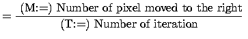 |
(9) |
[Ross,1983] Ross, S. (1983). Introduction to Stochastic Dynamic
The JAR-file of the applet (which can also be run as a stand-alone program)
is here.
The source code of the applet is here
(1 file).
The mathematical parts of this page are downloadable in PDF.
Reinforcement Learning
Repository : you will find there an excellent illustrated tutorial which
is mirrored here.
You can download A short Introdution to Reinforcement Learining
by Stephan ten Hagen and Ben Kröse.
The on-line book by Sutton
& Barto Book,"Reinforcement Learning: an introduction" is mirrored here.
A link to a Reinforcement
Learning site