System Identification
In GPC (Global Predictive Control) controllers
, we must simulate the process
to control. To preform the simulation we must first identify the system. There
are mainly three type of identification algorithms: global, structured and
local.
Global identification
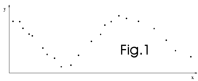
We start from the data (see fig.1 below):

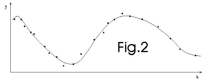
We use all the datas available to construct a global model (see fig. 2 below).
This technique is used, for example, in artificial neural network (NN) regressors.

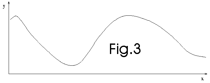
We discard the data. To make the prediction, we now only use the model (see
fig. 3 below):

This technique is used, for example, in artificial neural network (NN) regressors.
The NN is trained (often using gradient backpropagation) to fit the whole dataset.
Structural identification.
We, once again, start from the data (see fig 1 below):

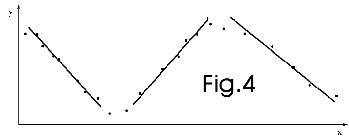
We perform a series of local fitting (see fig. 4 below). This technique is used,
for example, in Takagi-Sugeno fuzzy systems. Each rule of these systems correspond
to a part of the space. At each rule, there is a local model tailored for this
small part of the space. Thus, in the example below, there are 3 rules. The
quality of the prediction hardly depends on the number of rules. In the NLMIMO
toolbox, we use 10-fold cross-validation technique to find the optimal number
of rules. It's a very long process.

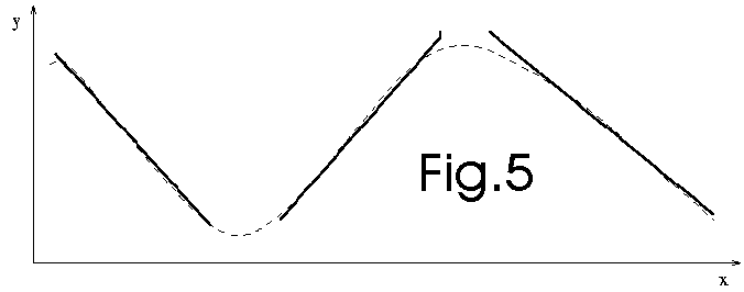
We discard the data. To make the prediction, we now only use the models (see
fig. 5 below):

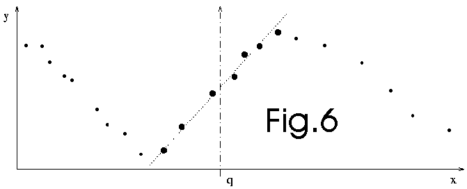
Local identification: The Lazy Learning approach.

Lazy learning postpones all the computation until an explicit request for
a prediction is received. The request is fulfilled by modelling locally the
relevant data stored in the database and using the newly constructed model
to answer the request. Each prediction requires therefore a local modelling
procedure. We will use, as regressor, a simple polynomial. The number of points
used for the construction of this polynomial (in other words, the kernel size
or the bandwidth) and the degree of the polynomial (0,1, or 2) are chosen
using leave-one out cross-validation technique. The identification of the
polynomial is performed using a recursive least square algorithm.
The cross-validation is performed at high speed using PRESS statistics.
What is leave-one out cross-validation? This is a technique used to evaluate
to quality of a regressor build on a dataset of  points. First, take
  points from the dataset (These points are the training set). The
last point
  will be used for validation purposes (validation set). Build the
regressor with the training set. Use this new regressor to predict the value
of the only point
  which has not been used during the building process. You obtain a
fitting error between the true value of
  and the predicted one. Continue, in a similar way, to build regressors,
each time on a different dataset of
  points. You obtain
  fitting errors for the
  regressors you have build. The global cross-validation error is the
mean of all these
  fitting errors.
We will choose the polynomial which has the lowest cross-validation error.
We can also give an estimate of the quality of the prediction: it's simply
the cross-validation error of the chosen model.
We can also choose the k polynomials
which have the lowest cross-validation error and use, as final model, a new
model which is the weighted average of these k
polynomials. The weight is the inverse of the cross-validation error. In the
Lazy learning toolbox, other possibilities of combination are possible.
The Lazy Learning requires a dataset in which the variance of the noise in
the data is locally constant. There can be a huge
noise on a small part of the data and nearly no noise everywhere else: This
is no problem. On the contrary, global identification tools like Neural Networks
demands that the variance of the noise in the data is globally
constant. This is why Lazy Learning performs nearly systematically
better than other classical global identification techniques.
Another advantage is the facility for on-line adaptation of the regressor.
In the case of Takagi-Sugeno fuzzy systems, each time we increase the training
set we have to wait several minutes for the computation of the new optimal
number of rules, the calculation of the new "places" for each rules
in the space and the construction of all the local models. On the contrary,
in the case of Lazy Learning, we only have to add one point inside the training
dataset. That's all. You can see here
an example of on-line adaptation with lazy learning.
One drawback of the lazzy learning approach is that it takes time to construct
at each query a good local model. Fortunately, most of the calculation time
is spend in the search of the neighbours points inside the dataset. For a
small dataset (less than 10000 points), the query is fullfilled immediatly
(no wait time on a P3 600 Mhz) (the search-loop has been highly optimized).
What to use and when ?
Suppose you want to identify some datas. What tool is the best for the job?
Bibliography
The excellent book
of Myers "Classical and Modern Regression With Applications" contains
all the mathematical demonstration used for the recursive least square
and the Press statistics.
For the implementation of these algorithms inside the Lazy Learning toolbox:
- "M. Birattari, G. Bontempi, and H. Bersini. Lazy learning meets the recursive
least-squares algorithm. In M. S. Kearns, S. A. Solla, and D. A. Cohn, editors,
Advances in Neural Information Processing Systems 11, Cambridge, 1999. MIT Press.",
available here.
- "Gianluca Bontempi and Mauro Birattari and Hugues Bersini, Recursive
Lazy Learning for Modeling and Control in "European Conference on Machine
Learning", pp 292-303, 1998", available here.
Download & Links
The first Lazy Learning toolbox : it's available for use with matlab at the
homepage of M.Birattari
.
The original algorithm has been nearly completely rewritten and forms now
a stand-alone package. The source code is available here.
It is pure C/C++ code which compiles on both windows and unix. The search
inside the dataset has been accelerated. You can now re-configure the parameters
"on the fly". The Object Oriented approach allows a better comprehention
of the algorithm. There is a small example file "testSetGen.cpp"
which demonstrate the toolbox. You will find inside this
paper informations on how to use the classes.
