Trust Region Algorithms

The algorithm decribed here is a simplification of the one used in my thesis (1). So, for more information, see the thesis

.

I will give an example based on the optimization (minimization) of the following function:

We start our research from the point (0.7; -3.3). The current point

is always the red dot in the figures below. k will always be the iteration index.

We want an algorithm which make the least possible number of function evaluations. Of course, to build a figure like the ones below, we evaluate the objective function a huge number of time. If you are able to construct such figure, it means that your objective function is very cheap to evaluate and you might consider using an other algorithm: the rosenbrock method.

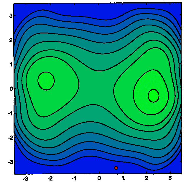
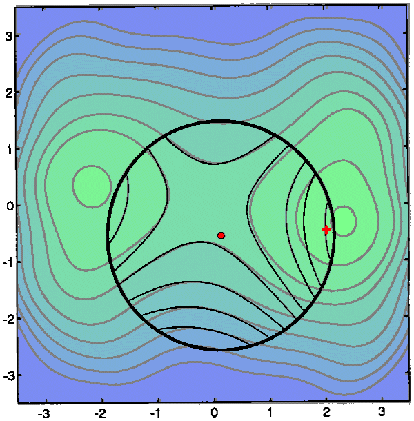
We will construct a local approximation Q(x) of f(x) around . Q(x) is a polynomial of degree 2. Q(x) is represented in the figure below with bold lines. We will define a Trust Region around the current point . The trust region is a disc of radius centered at .We will search for the minimum of Q(x) inside the Trust Region. This minimum is the red cross in the figures below.

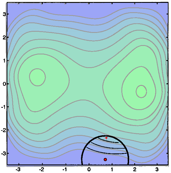
We obtain < : this is a success: Q(x) is a good local approximator of f(x) and has given us a good advice. We will move the current position to and iterate (k:=k+1). Since Q(x) is so good we will also increase the trust region radius . We will re-contruct a new quadratic interpolation Q(x) around the new . This re-construction can induce many evaluation of the objective function. In fact, in most optimization algorithms, this is where the greatest number of function evaluations are spend. In the algorithm developped, I use a special heuristic due to powel(2) to reduce the re-construction cost. This heuristic is based on Multivariate Lagrange Interpolation Polynomials. There are also other possibilities to construct Q(x) like the BFGS method. 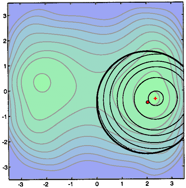See the figure below for a graphical explanation of the second step of the algorithm. (the red cross) is once again the minimum of Q inside the Trust Region.

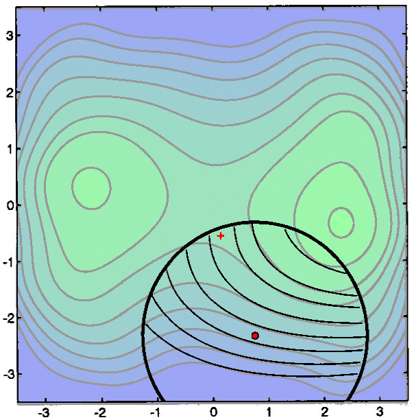
We obtain, once again, a success: < . We move to the new position.We Reconstruct Q(x).
We Increase .

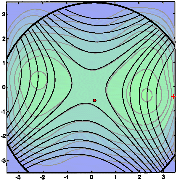
This will be a failure: > . Q(x) is not anymore a correct approximation of f(x). We thus reduce . The current position is not changed.

This is a partial success: < but the reduction is not as big as predicted by Q(x), so we do not change . The current position is moved.

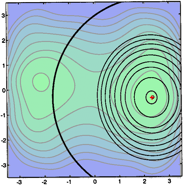
The next iterations do not exhibit anything new. Note that the trust region radius is becoming very huge at the end of the search. We stop when the step size (=|| - ||) is becoming too small

.

Bibliography

(1) Frank Vanden Berghen, Thesis on Continous optimization is available here. The on-line version is available here.
(2) Powel, UOBYQA: unconstrained optimization by quadratic optimization.

Download

My thesis on Continous optimization is available here(or on-line version). It's a stand-alone book designed to be read by graduate students with no a-priori knowledge in the optimization field.

The code of my optimizer is here. It's a complete C/C++ stand-alone package. You can compile it under unix or windows, there is no special library needed. It is completely written in C/C++ in pure structural programmation style (no 'goto' instruction). The code has been highly optimized (with extend use of memcpy function, special fast matrix manipulation and so on...). It's easily comprehensible since the whole complex algorithm is cutted into simple objects. There is a small example (file 'Main.cpp') to show how to use the package. The whole code is described in my thesis