


Next: Non-Linear constraints
Up: A short review of
Previous: A short review of
Contents
Subsections
We want to find


 which satisfies:
where  is the dimension of the search space and
  is the
number of linear constraints.
The material of this section is based on the following reference:
[Fle87].
is the
number of linear constraints.
The material of this section is based on the following reference:
[Fle87].
Figure 8.1:
Violation of a constraint.
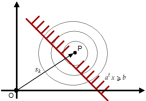 |
At each step  computed from 8.1, we check if one
of the linear constraints has been violated. On the figure
8.1, the linear constraint
computed from 8.1, we check if one
of the linear constraints has been violated. On the figure
8.1, the linear constraint
 has been
violated and it's thus "activated". Without loosing generality,
let's define
has been
violated and it's thus "activated". Without loosing generality,
let's define
 and
and
 the set of the
  active constraints.
Figure 8.2:
A search in the reduced space of the active
constraints gives as result 
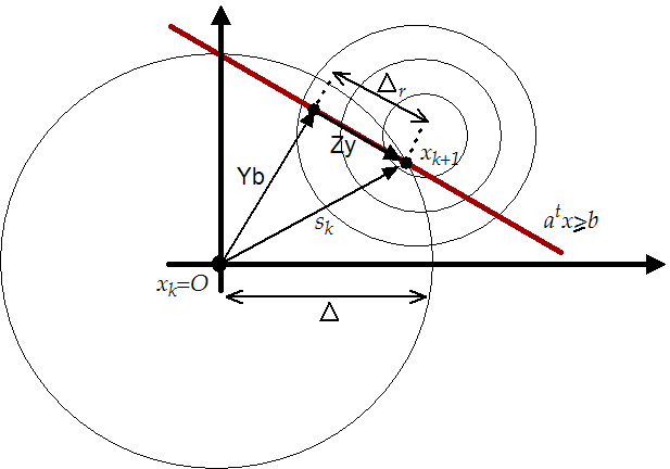 |
Let  and
and  be
be
 and
and
 matrices
respectively such that
matrices
respectively such that ![$ [Y:Z]$](img917.png) is non-singular, and in addition
let
is non-singular, and in addition
let  and
and  . The step must be feasible, so we must
have to
. The step must be feasible, so we must
have to
 . A solution to this equation is given by:
 where can be any vector. Indeed, we have the
following:
where can be any vector. Indeed, we have the
following:
 .
The situation is illustrated in figure 8.2. We will
choose as the solution of
.
The situation is illustrated in figure 8.2. We will
choose as the solution of
 subject to subject to  |
(8.4) |
with
 . In other words, is the
minimum of the quadratical approximation of the objective function
limited to the reduced space of the active linear constraints and
limited to the trust region boundaries. We have already developed
an algorithm able to compute in chapter 4.
. In other words, is the
minimum of the quadratical approximation of the objective function
limited to the reduced space of the active linear constraints and
limited to the trust region boundaries. We have already developed
an algorithm able to compute in chapter 4.
When using this method, there is no difference between "
approach 1" and "approach 2".
This algorithm is very stable in regards to rounding error. It's
very fast because we can make Newton step (quadratical convergence
speed) in the reduced space. Beside, we can use software developed
in chapter 4. For all these reasons, it has been chosen
and implemented. It will be fully described in chapter
9.
The material of this section is based on the following reference:
[CGT00e].
In these methods, we will follow the "steepest descent steps": we
will follow the gradient. When we enter the infeasible space, we
will simply project the gradient into the feasible space. A
straightforward (unfortunately false) extension to this technique
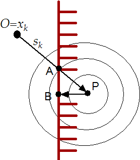
is the "Newton step projection algorithm" which is illustrated in
figure 8.3. In this figure the current point is  .
The Newton step () lead us to point P which is infeasible.
We project P into the feasible space: we obtain B. Finally, we
will thus follow the trajectory OAB, which seems good.
.
The Newton step () lead us to point P which is infeasible.
We project P into the feasible space: we obtain B. Finally, we
will thus follow the trajectory OAB, which seems good.
Figure 8.3:
"newton's step projection algorithm" seems
good.
 |
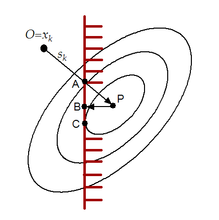
In figure 8.4, we can see that the "Newton step
projection algorithm" can lead to a false minimum. As before, we
will follow the trajectory OAB. Unfortunately, the real minimum of
the problem is C.
Figure 8.4:
"newton's step projection algorithm" is
false.
 |
We can therefore only follow the gradient,not the Newton step. The
speed of this algorithm is thus, at most, linear, requiring many
evaluation of the objective function. This has little consequences
for "approach 1" but for "approach 2" it's
intolerable. For these reasons, the Null-space method seems more
promising and has been chosen.
Next: Non-Linear constraints
Up: A short review of
Previous: A short review of
Contents
Frank Vanden Berghen
2004-04-19