


Next: The SQP algorithm
Up: Detailed description of the
Previous: Detailed description of the
Contents
Subsections
The material of this section is based on the following reference:
[Fle87].
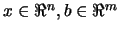
We want to find the solution of:
 subject to subject to  |
(9.1) |
where
 and
and
 .
.
We will assume in this chapter that  is positive definite.
There is thus only one solution. We will first see how to handle
the following simpler problem:
is positive definite.
There is thus only one solution. We will first see how to handle
the following simpler problem:
subject to  |
(9.2) |
Equality constraints
Let  and
and  be
be
 and
and
 matrices
respectively such that
matrices
respectively such that ![$ [Y:Z]$](img917.png) is non-singular, and in addition
let
is non-singular, and in addition
let  and
and  . The solution of the equation
  is
given by:
is
given by:
 |
(9.3) |
where  can be any
vector. Indeed, we have the following:
can be any
vector. Indeed, we have the following:
 . The matrix has linearly independent columns
 which are inside the null-space of
  and
therefore act as bases vectors (or reduced coordinate directions)
for the null space. At any point
and
therefore act as bases vectors (or reduced coordinate directions)
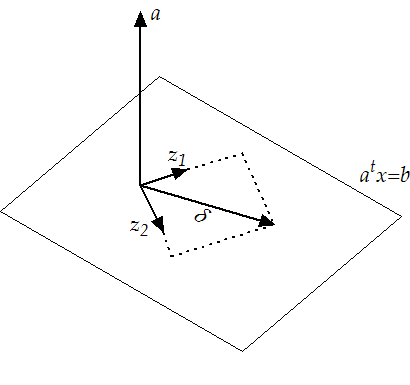
for the null space. At any point  any feasible correction
 can be written as:
 |
(9.4) |
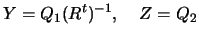
where
 are the components (or reduced
variables) in each reduced coordinate direction (see Figure
9.1).
are the components (or reduced
variables) in each reduced coordinate direction (see Figure
9.1).
Figure 9.1:
The null-space of A
 |
Combining equation 9.2 and 9.3, we obtain the
reduced quadratic function:
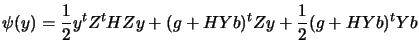 |
(9.5) |
If  is positive definite then a minimizer
  exists which solves
the linear system:
exists which solves
the linear system:
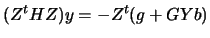 |
(9.6) |
The
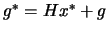
solution is computed using Cholesky factorization. Once
is known we can compute  using equation 9.3
and
using equation 9.3
and  using the secant equation 13.29:
 . Let's recall equation 13.19:
 |
(9.7) |
Let's now
compute  : From equation 9.7 we have:
 |
(9.8) |
Pre-Multiply 9.8 by
 and using
  , we have:
 |
(9.9) |
Depending on the choice of and , a number of methods exist.
We will obtain and from a QR factorization of the matrix
 (see annexe for more information about the QR factorization
of a matrix). This can be written:
(see annexe for more information about the QR factorization
of a matrix). This can be written:
![$\displaystyle A^t= Q \left[
\begin{array}{c} R
\\ 0 \end{array} \right] = \l...
..._1 \; Q_2 \right] \left[
\begin{array}{c} R \\ 0
\end{array} \right] = Q_1 R$](img1115.png) |
(9.10) |
where
 is an orthogonal matrix,
 is an upper triangular matrix,
 and
and
 . The choices
 |
(9.11) |
have the correct
properties. Moreover the vector  in equation 9.3
and figure 9.2 is orthogonal to the constraints. The
reduced coordinate directions
in equation 9.3
and figure 9.2 is orthogonal to the constraints. The
reduced coordinate directions  are also mutually orthogonal.
is calculated by forward substitution in
are also mutually orthogonal.
is calculated by forward substitution in  followed
by forming
followed
by forming  . The multipliers are calculated
by backward substitution in
. The multipliers are calculated
by backward substitution in
 .
.
Figure 9.2:
A search in the reduced space of the active
constraints give as result
 |
Certain constraints, indexed by the Active set  , are
regarded as equalities whilst the rest are temporarily
disregarded, and the method adjusts this set in order to identify
the correct active constraints at the solution to 9.1.
Each iteration attempts to locate the solution to an Equality
Problem (EP) in which only the active constraints occur. This is
done by solving:
, are
regarded as equalities whilst the rest are temporarily
disregarded, and the method adjusts this set in order to identify
the correct active constraints at the solution to 9.1.
Each iteration attempts to locate the solution to an Equality
Problem (EP) in which only the active constraints occur. This is
done by solving:
subject to 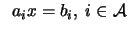 |
(9.12) |
Let's define, as usual,
 . If
. If  is infeasible then the length
  of the
step is chosen to solve:
of the
step is chosen to solve:
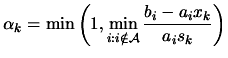 |
(9.13) |
If
 then a new
constraint becomes active, defined by the index which achieves the
min in 9.13, and this index is added to the active
set
then a new
constraint becomes active, defined by the index which achieves the
min in 9.13, and this index is added to the active
set  . Suppose we have the solution of the EP. We
will now make a test to determine if a constraint should become
inactive. All the constraints which have a negative associated
Lagrange multiplier
. Suppose we have the solution of the EP. We
will now make a test to determine if a constraint should become
inactive. All the constraints which have a negative associated
Lagrange multiplier  can become inactive. To summarize
the algorithm, we have:
can become inactive. To summarize
the algorithm, we have:
- Set
 a feasible
point.
a feasible
point.
- Solve the EP.
- Compute the Lagrange multipliers
 . If
. If
 for all constraints then terminate. Remove the constraints
which have negative .
for all constraints then terminate. Remove the constraints
which have negative .
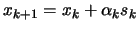
- Solve 9.13 and activate a new constraint if
necessary.
- set
 and go to (2).
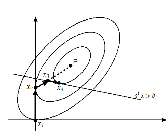
An illustration of the method for a simple QP problem is shown in
figure 9.3. In this QP, the constraints are the
bounds  and a general linear constraint
 .
.
Figure 9.3:
Illustration of a simple QP
 |
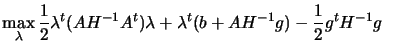
If is positive definite, the dual of (
 )
)
 subject
to subject
to |
(9.14) |
is given by
 subject to subject to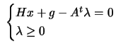 |
(9.15) |
By eliminating from the first constraint
equation, we obtain the bound constrained problem:
 subject to subject to |
(9.16) |
This problem can be solved by means of the gradient projection
method, which normally allows us to identify the active set more
rapidly than with classical active set methods. The matrix
 is semi-definite positive when is positive
definite. This is good. Unfortunately, if we have linearly
dependent constraints then the matrix
becomes
singular (this is always the case when
is semi-definite positive when is positive
definite. This is good. Unfortunately, if we have linearly
dependent constraints then the matrix
becomes
singular (this is always the case when  ). This lead to
difficulties when solving 9.16. There is, for example,
no Cholesky factorization
possible.
). This lead to
difficulties when solving 9.16. There is, for example,
no Cholesky factorization
possible.
My first algorithm used gradient projection to identify the active
set. It then project the matrix
into the space of
the active constraints (the projection is straight forward and
very easy) and attempt a Cholesky factorization of the reduced
matrix. This fails very often. When it fails, it uses "steepest
descent algorithm" which is sloooooooow and useless. The final
implemented QP works in the primal space and use QR
factorization to do the projection.
The QP which has been implemented uses normalization techniques on
the constraints to increase robustness. It's able to start with an
infeasible point. When performing the QR factorization of ,
it is using pivoting techniques to improve numerical stability. It
has also some very primitive technique to avoid cycling. Cycling
occurs when the algorithm returns to a previous active set in the
sequence (because of rounding errors). The QP is also able to
"warm start". "Warm start" means that you can give to the QP an
approximation of the optimal active set . If the given
active set and the optimal active set
 are close, the
solution will be found very rapidly. This feature is particularly
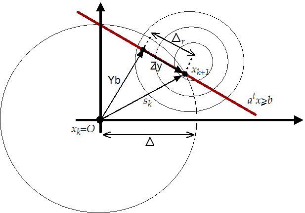
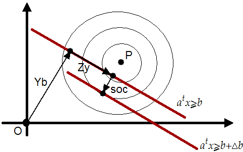
useful when doing SQP. The code can also compute very efficiently
"Second Order Correction steps" (SOC step) which are needed for
the SQP algorithm. The SOC step is illustrated in figure
9.4. The SOC step is perpendicular to the active
constraints. The length of the step is based on
are close, the
solution will be found very rapidly. This feature is particularly
useful when doing SQP. The code can also compute very efficiently
"Second Order Correction steps" (SOC step) which are needed for
the SQP algorithm. The SOC step is illustrated in figure
9.4. The SOC step is perpendicular to the active
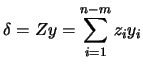
constraints. The length of the step is based on  which
is calculated by the SQP algorithm. The SOC step is simply
computed using:
which
is calculated by the SQP algorithm. The SOC step is simply
computed using:
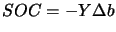 |
(9.17) |
Figure 9.4:
The SOC step
 |
The solution to the EP (equation 9.12) is computed in one
step using a Cholesky factorization of . This is very fast but,
for badly scaled problem, this can lead to big rounding errors in
the solution. The technique to choose which constraint enters the
active set is very primitive (it's based on equation
9.13) and can also lead to big rounding errors. The
algorithm which finds an initial feasible point when the given
starting point is infeasible could be improved. All the
linear algebra operations are performed with dense matrix.
This QP algorithm is very far from the "state-of-the-art". Some
numerical results shows that the QP algorithm is really the weak
point of all the optimization code. Nevertheless, for most
problems, this implementation gives sufficient results (see
numerical results).
Next: The SQP algorithm
Up: Detailed description of the
Previous: Detailed description of the
Contents
Frank Vanden Berghen
2004-04-19